We already saw that there is a natural way to put many polynomial continued fraction in a single interesting structure called a conservative matrix field. Recall that a (2-dimensional) conservative matrix field consists of two matrices \(M_X(x,y), M_Y(x,y)\) such that
- Both \( M_X(x,y) \) and \( M_Y(x,y) \) are polynomial in \( x,y \).
- It is conservative, namely for any \((x,y)\) we have that
\( M_Y(x,y) \cdot M_X(x, y+1) = M_X(x,y) \cdot M_Y( x+1,y) \).
Our original search for polynomial continued fractions related to \(\zeta(3)\) led us to this construction, and we will now see how to build many more such matrix fields.
The \(f,\bar{f} \) construction
For the construction of the next matrix field, we will need two polynomials \(f(x,y),\bar{f}(x,y)\). We say that these polynomials are conjugated if they satisfy these two interesting conditions:
Linear condition:
For any \(x,y\) they satisfy:
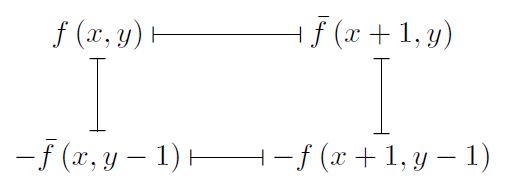
\(f(x,y) – \bar{f}(x+1,y) = f(x+1,y-1) – \bar{f}(x,y-1)\).
In case this holds, we will denote the expression above by \(a(x,y)\).
Quadratic condition:
For any \(x,y\) they satisfy:
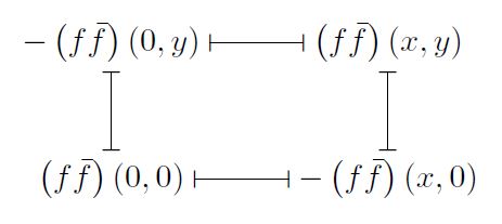
\((f\bar{f})(x,y) – (f\bar{f})(0,y) = (f\bar{f})(x,0) – (f\bar{f})(0,0) \).
Here we will denote the expression above by \(b(x)\), and in particular note that it is only a function of \(x\).
Remark: There are many solutions to these two conditions, but before we show them, let us note a few observations about them:
- If we start with two generic polynomials, namely \(f(x,y) = \sum_{i,j=1}^d a_{i,j}x^i y^j, \; f(x,y) = \sum_{i,j=1}^d \bar{a}_{i,j}x^i y^j\), then solving the linear and quadratic conditions above will lead to a linear and quadratic system of equations respectively in the \(a_{i,j}, \bar{a}_{i,j}\).
- The linear condition can be seen as an equation about the evaluations of \(f,\bar{f}\) over the four corners of a square, where their sum needs to be zero:
- Similarly, the quadratic condition can also be seen as equation of evaluations of \((f\bar{f})(x,y)\) over the 4 corners of a square.
- Finally, writing down \((f\bar{f})(x,y)=\sum b_{i,j} x^i y^j \), the quadratic condition simply says that the mixed monomials are zero, namely \(b_{i,j}=0\) whenever both \(i,j>0\).
The matrix field construction
If \(f,\bar{f}\) are conjugated polynomials, then
\(M_X(x,y)=\begin{pmatrix}0 & b(x)\\1 & a(x,y)\end{pmatrix}\)
\(M_Y(x,y)=\begin{pmatrix}\bar{f}(x,y) & b(x)\\1 & f(x,y)\end{pmatrix}\)
form a conservative matrix field.
We already saw one matrix field using this construction, when we looked at polynomial continued fractions for \(\zeta(3)\). In that case our polynomials were \(f(x,y)=\frac{y^3-x^3}{y-x} (y+x) = x^3 + 2x^2y + 2xy^2 + y^3\) and \(\bar{f}(x,y)=f(-x,y)\). While this was not a requirement, it is interesting to note how closely related \(f\) and \(\bar{f}\) are here, in the sense that the second is the image of the first under the simple homomorphism which maps \( x\mapsto -x \).
In general, these constructions not only produce many matrix fields, but every horizontal line corresponds to a polynomial continued fraction, namely \(M_X(k,y_0)\) for \(y_0\) fixed. Moreover, considering the \(y_0=1\) case, we get:
\(M_X(x,1)= \begin{pmatrix}0 & b(x)\\1 & a(x,1)\end{pmatrix}= \begin{pmatrix}0 & f(x,0)\bar{f}(x,0)\\1 & f(x+1,0) – \bar{f}(x,0)\end{pmatrix}\).
This type of polynomial continued fraction was the simple form that can be directly related to infinite sums using Euler’s conversion formula. With this in mind, when speaking about a matrix field using this construction, when possible we will add the value of this continued fraction (up to a Mobius transformation) arising from the first line.
Some sporadic examples
We start with a few examples corresponding to some interesting constants.
- \(\ln(2)\) corresponds to the construction using \(f(x,y)=x+y\; , \; \bar{f}(x,y)=f(x,-y)=x-y\).
- \(e\) corresponds to the construction using \(f(x,y)=x+y \; , \; \bar{f}(x,y)=1\).
- \(\pi\) corresponds to the construction using \(f(x,y)= 1+2(x+y) \; , \; \bar{f}(x,y) = y-x \).
- \(\zeta(2)\) corresponds to the construction using \( f(x,y)=2x^2 + 2xy + y^2\; , \; \bar{f}(x,y)=-f(-x,y) \).
- \(\zeta(3)\) corresponds to the construction using \( f(x,y)=\frac{y^3-x^3}{y-x} (y+x) , \; \bar{f}(x,y)=f(-x,y) \).
The degree 1 case
In the case where both \(f\) and \(\bar{f}\) are of degree 1, we can give a full mathematical solution to the linear and quadratic condition. In particular, writing
\(f(x,y)= ax + by + c \; ; \; \bar{f}(x,y) = \bar{a}x + \bar{b}y + \bar{c} \),
the conditions above translate to:
Linear condition: \( b-a = \bar{b}+\bar{a} \)
Quadratic condition: \( a\bar{b} + \bar{a}b = 0 \)
These two together lead to two families of conservative matrix field. The first one is
\( f(x,y) = a(x+y) + c ; \bar{f}(x,y) = \bar{a}(x-y) + \bar{c} \),
and the second is
\( f(x,y) = ax + by + c ; \bar{f}(x,y) =-ax + by + \bar{c} \)
The degree 2 case
In the cases where \(f\) and \(\bar{f}\) are of higher degree, the linear and quadratic condition yield a more complicated set of restrictions between the coefficients. Solving for it numerically gives the following form for \(f\) and \(\bar{f}\):
\(
f(x,y) = (2c_1 + c_2)(c_1 + c_2) – c_3 c_0 – c_3 ((2c_1 + c_2) (x+y) + (c_1 + c_2)(2x + y)) + c_3^2 (2x^2 + 2xy + y^2)
\\\\
\bar{f}(x,y) = c_3 (c_0 + c_2 x + c_1 y – c_3 (2x^2 – 2xy + y^2))
\)
For example, by substituting \(\vec{c} = (0,0,0,1)\) we get the conservative matrix field for \(\zeta(2)\). This conservative matrix field also creates formulas for Catalan’s constant!
The degree 3 case
Now, the linear and quadratic condition take into account even more coefficients, making solving them a harder problem, which was not feasible using standard computation power. By setting the constant coefficient in \(f\) and \(\bar{f}\) to be zero, a numerical solution yield three possible structures:
\(
f_1(x,y) = -((c_0+c_1 (x+y))(c_0 (x+2 y)+c_1 (x^2+x y+y^2 ))) \\\\
\bar{f_1}(x,y) = (c_0+c_1 (-x+y))(c_0 (x-2 y)-c_1 (x^2-x y+y^2 ))
\)
\(
f_2(x,y) = (c_0+c_1 (-x+y))(c_0 (x-2 y)-c_1 (x^2-x y+y^2 )) \\\\
\bar{f_2}(x,y) = (c_0+c_1 (-x+y))(c_0 (x-2 y)-c_1 (x^2-x y+y^2 ))
\)
\(
f_3(x,y) = (x+y)(c_0^2-c_0 c_1 (x-y)-2 c_1^2 (x^2+x y+y^2 )) \\\\
\bar{f_3}(x,y) = (c_0+c_1 (x-y))(3 c_0 (x-y)+2 c_1 (x^2-x y+y^2 ))
\)
For example, by substituting \(\vec{c} = (0,1)\) we get the conservative matrix field for \(\zeta(3)\), which can also be used to prove it’s irrationality!
Other choices of \(\vec{c}\) can also create a conservative matrix field for \(\pi^3\)