At this point we know that there are many polynomial continued fractions, and there are all sorts of ways to generate them (see here for example). Our next step is to try to combine them together into a larger structure which will allow us to extract all sorts of interesting results about them.
To fix our notation, recall that:
\( \mathbb{K}_1^n\frac{b_k}{a_k} = \frac {b_1}{a_1+ \frac{b_2}{a_2 + \frac{b_3}{\ddots + \frac{b_n}{a_n}}}},\)
and we also have the Mobius transformation notation:
\( \mathbb{K}_1^n\frac{b_k}{a_k} = \begin{pmatrix}0 & b_1\\1 & a_1\end{pmatrix} \cdots \begin{pmatrix}0 & b_n\\1 & a_n\end{pmatrix}(0)\)
where in general
\( \begin{pmatrix}a & b\\c & d\end{pmatrix} (z) = \frac{az+b}{cz+d}.\)
Many expansions, same convergents
In the realm of simple continued fraction expansions, every irrational number \(\alpha\) possesses a unique expansion (while rationals have exactly two expansions). However, when it comes to polynomial continued fractions, a single constant can have many expansions. This prompts us to explore the process of transitioning between different expansions of the same number \(\alpha\).
One approach to discovering distinct expansions for \(\alpha \), involves traversing through different (rational) representations of the convergents that converge to \(\alpha\). For instance, even in the initial step in the polynomial continued fraction, we can transition between various forms, such as:
\( \begin{pmatrix}0 & b_1\\1 & a_1\end{pmatrix} (0) = \frac{b_1}{a_1} = \frac{c_1 b_1}{c_1 a_1}=\begin{pmatrix}0 & c_1 b_1\\1 & c_1 a_1\end{pmatrix} (0) =\begin{pmatrix}0 & b_1\\1 & a_1\end{pmatrix} \begin{pmatrix}1 & 0\\0& c_1\end{pmatrix} (0) .\)
More generally, given two expansions for the same number \(\mathbb{K}_1^\infty\frac{b_k}{a_k} = \alpha = \mathbb{K}_1^\infty\frac{b_k’}{a_k’} \) where the convergents are the same, namely \(\mathbb{K}_1^n\frac{b_k}{a_k} = \alpha = \mathbb{K}_1^n\frac{b_k’}{a_k’} \) for all \(n\), a simple induction will show that the expansions are equivalent, namely
\( \mathbb{K}_1^\infty \frac{b_k}{a_k} = \frac{1}{c_0}\mathbb{K}_1^\infty \frac{c_{k-1}c_k b_k}{c_k a_k} \).
In the Mobius notation, we get that
\( \left[ \prod_1^n \begin{pmatrix}0 & b_k\\1 & a_k\end{pmatrix} \right] (0) = \frac{1}{c_0} \left[\prod_1^n \begin{pmatrix}c_{k-1} & 0\\0 & 1\end{pmatrix} \begin{pmatrix}0 & b_k\\1 & a_k\end{pmatrix} \begin{pmatrix}1 & 0 \\0 & c_k\end{pmatrix} \right] (0) \)
Coboundary equivalence
The last example suggests an interesting construction. Let \( M_k \) be our polynomial continued fraction matrices, and let \( U_k \) be another sequence of invertible matrices for \( k\geq 0\), and we consider the new “Mobius continued fraction” defined by:
\( \displaystyle{\lim_{n\to \infty}}\left[\prod_1^n U_{k-1}^{-1} M_k U_k \right] (0) = \displaystyle{\lim_{n\to \infty}} U_0 ^{-1} \left[\prod_1^n M_k \right] U_n (0)\).
In the example above we take \( U_k = \begin{pmatrix}1 & 0 \\0 & c_k\end{pmatrix} \). Since we are only interested in the Mobius transformation, two matrices which differ by scalar multiplication define the same Mobius transformation, and we think of them as equivalent. In particular, we get that \(U_{k-1}^{-1} \sim \begin{pmatrix}c_{k-1} & 0 \\0 & 1\end{pmatrix} \), so in this sense, the product on the right is of matrices of the form \( U_{k-1}^{-1} M_k U_k \).
What can we say about this new “Mobius continued fraction” and its connection to the original limit of \( \left[\prod_1^n M_k \right] (0) \)? In particular, if \( M_k = \begin{pmatrix}0 & b(k)\\1& a(k)\end{pmatrix} \) has a polynomial continued fraction from, and \( U_{k-1}^{-1} M_k U_k \) also has polynomial continued fraction from, what can we say about both limits?
We call this type of “increasing indexed conjugation”, namely the map \( M_k \mapsto U_{k-1}^{-1} M_k U_k\) a coboundary equivalence. This name came from homology theory, though we will not go into the deeper parts of this theory, and will just keep the name.
In general, given two polynomial matrices \(M(x), M'(x)\), it is not clear how to find if they are coboundary equivalent via a polynomial matrix \(U(x)\), namely \(M(x)U(x+1)=U(x)M'(x)\). However, if we bound the degree of the polynomials in \(U(x)\), then this problem becomes a simple system of linear equations. As such we provide this python program where you can check whether two such polynomial matrices are coboundary equivalent.
The \(\zeta(3)\) example
To understand this concept, lets start with an interesting example of a family of polynomial continued fractions related to \(\zeta(3)\). As we saw here, the standard rational approximation for \(\zeta(3)\), namely \(\frac{p_n}{q_n} := \sum_{k=1}^n \frac{1}{k^3} \) can be written in a polynomial continued fraction (PCF) form as follows
\( \frac{p_n}{q_n} = \frac{1}{1+\mathbb{K}_1^n \frac{k^{-6}}{k^3 + (k+1)^3}}=\begin{pmatrix}0 & 1\\1& 1\end{pmatrix}\cdot \left[ \prod_1^n \begin{pmatrix}0 & k^{-6}\\1& k^3 + (k+1)^3\end{pmatrix} \right] (0)\),
or alternatively we have
\(\frac{1}{\zeta(3)} = 1+\mathbb{K}_1^n \frac{k^{-6}}{k^3 + (k+1)^3} = (0^3+1^3)+\mathbb{K}_1^n \frac{k^{-6}}{k^3 + (k+1)^3}\).
As it turns out, the matrix \( M_k = \begin{pmatrix}0 & k^{-6}\\1& k^3 + (k+1)^3\end{pmatrix} \) can be (coboundary) conjugated into a second interesting polynomial continued fraction. More specifically, we have:
\( U_k = \begin{pmatrix}\frac{1+k^3}{1+k} (1-k) & k^{-6}\\1& \frac{1-k^3}{1-k} (1+k) \end{pmatrix} \),
\( U_{k-1}^{-1} M_k U_k = \begin{pmatrix}0 & k^{-6}\\1& k^3 + (k+1)^3 + 4(2k+1)\end{pmatrix} \).
Even more interestingly, the limit of \( U_0^{-1} \left[ \prod _1^n M_k \right] U_n (0) \) converges to
\(\frac{1}{\zeta(3)-1} = (0^3+1^3+4(2\cdot 0 + 1))+\mathbb{K}_1^n \frac{k^{-6}}{k^3 + (k+1)^3 + 4(2k+1)}\).
Can we do it a second time and get another polynomial continued fraction with limit that relates to \( \zeta(3) \)? Is there a fourth and fifth and sixth such layers? It appears that there are, and more over moving from one layer to the next is also done in an intriguing way.
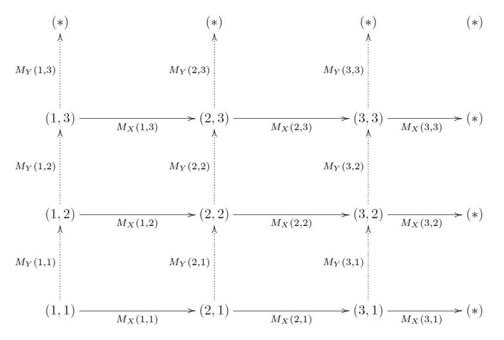
The matrices \( M_X(x,1) \) on the bottom line correspond to our “standard” \(\zeta(3)\) expansion, namely \( \mathbb{K}_1^\infty \frac{-k^6}{k^3+(k+1)^3}\).
The matrices \( M_X(x,2) \) on the second line gives us the second polynomial continued fraction from above \( \mathbb{K}_1^\infty \frac{-k^6}{k^3+(k+1)^3 + 4(2k+1)}\).
More generally, on the \( m\)‘th line, we get the polynomial continued fraction \( \mathbb{K}_1^\infty \frac{-k^6}{k^3+(k+1)^3 + 2m(m-1)(2k+1)}\) and the limit is \( \frac{1}{\sum_m^{\infty} \frac{1}{n^3}} – (1 + 2m(m-1)) \).
More interestingly, the conjugating matrix between the first and second line is non other that \( U_k = M_Y(k, 1) \), or more generally we get that
\( M_X(x, 2) = M_Y(x,1)^{-1} M_X(x,1) M_Y( x+1,1) \),
which we can also write as
\( M_Y(x,1) M_X(x, 2) = M_X(x,1) M_Y( x+1,1) \).
This continues on to any line, and in general we get this interesting property
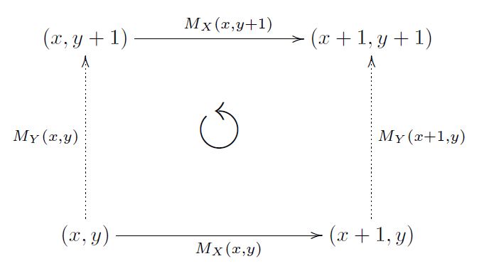
\( M_Y(x,y) M_X(x, y+1) = M_X(x,y) M_Y( x+1,y) \),
We can view this property as a conservativeness property (as in conservative vector fields): if we start at position \((x,y)\) and then go right and then up, or up and then right, then multiplying the matrices along the way gives you the same result. In other words, we have the following commutative diagram:
We now have an interesting new structure where (1) The limit of the polynomial at each horizontal line \(y\) is (more or less) \(\sum_y^{\infty} \frac{1}{n^3}\) and (2) multiplying the matrices along a given path, is only a function of the two endpoints. Further investigation into this structure can reveal many more interesting phenomena, but at the very least, it leads us to the next interesting definition:
Definition ( The conservative matrix field ):
A conservative (2-dimensional) matrix field consists of two matrices \(M_X(x,y), M_Y(x,y)\) such that
- Both \( M_X(x,y) \) and \( M_Y(x,y) \) are polynomial in \( x,y \).
- It is conservative, namely for any \((x,y)\) we have that
\( M_Y(x,y) \cdot M_X(x, y+1) = M_X(x,y) \cdot M_Y( x+1,y) \).
As we can see above, this definition has at least one object satisfying it, however, there are many more such matrix fields that we shall describe here, which correspond to other constants in the same way that this one corresponds to \(\zeta(3)\).